Memory Customization

Author: Yi-Hsiang Lai (seanlatias@github)

In this tutorial, we demonstrate how memory customization works in HeteroCL.

import heterocl as hcl
import numpy as np

Memory Customization in HeteroCL

There are two types of memory customization in HeteroCL. The first one is similar to what we have seen in Compute Customization, where we demonstrate some primitives that will be synthesized as pragmas. An example of such primitive is partition. Following is an example. Note that the primitive is directly applied on the schedule instead of a stage. This is because we are modifying the property of a tensor.

hcl.init()

A = hcl.placeholder((10, 10), "A")

def kernel(A):
    return hcl.compute(A.shape, lambda x, y: A[x][y]+1, "B")

s = hcl.create_schedule(A, kernel)
s.partition(A)
print(hcl.lower(s))

Out:

array partition variable=A complete factor=0 dim=0
// attr [_top] storage_scope = "global"
allocate _top[int32 * 1]
produce _top {
  // attr [0] extern_scope = 0
  produce B {
    // attr [0] extern_scope = 0
    for (x, 0, 10) {
      for (y, 0, 10) {
        B[(y + (x*10))] = (A[(y + (x*10))] + 1)
      }
    }
  }
}

In the IR, we should see a line that annotates tensor A to be partitioned completely.

Note

For more information, please see heterocl.schedule.Schedule.partition

Another example is to reshape a tensor. This is helpful when we combine partitioning with loop titling. In this example, we split the inner axis y and also reshape the output tensor B. After that, we pipeline the middle axis yo and partition the output tensor accordingly. Note that the reshape primitive cannot be applied to the input tensors.

hcl.init()

s = hcl.create_schedule(A, kernel)
yo, yi = s[kernel.B].split(kernel.B.axis[1], 5)
s[kernel.B].pipeline(yo)
s.reshape(kernel.B, (10, 2, 5))
s.partition(kernel.B, dim=3)
print(hcl.build(s, target="vhls"))

Out:

#include <ap_int.h>
#include <ap_fixed.h>
#include <hls_stream.h>
#include <math.h>
#include <stdint.h>
void default_function(ap_int<32> A[10*10], ap_int<32> B[10*2*5]) {
  ap_int<32> _top;
  #pragma HLS array_partition variable=B complete dim=3
  for (ap_int<32> x = 0; x < 10; ++x) {
    for (ap_int<32> y_outer = 0; y_outer < 2; ++y_outer) {
    #pragma HLS pipeline
      for (ap_int<32> y_inner = 0; y_inner < 5; ++y_inner) {
        B[((y_inner + (y_outer * 5)) + (x * 10))] = (A[((y_inner + (y_outer * 5)) + (x * 10))] + 1);
      }
    }
  }
}

Data Reuse in HeteroCL

The other type of memory customization primitives involves the introduction of allocation of new memory buffers. An example is data reuse. The idea of data reuse is to reduce the number of accesses to a tensor by introducing an intermediate buffer that holds the values being reused across different iterations. This finally leads to better performance in hardware.

Example: 2D Convolution

To demonstrate this, we use the computation of 2D convolution as an example. Let’s see how we can define 2D convolution in HeteroCL.

hcl.init()

A = hcl.placeholder((6, 6), "A")
F = hcl.placeholder((3, 3), "F")

def kernel(A, F):
    r = hcl.reduce_axis(0, 3)
    c = hcl.reduce_axis(0, 3)
    return hcl.compute((4, 4),
            lambda y, x: hcl.sum(A[y+r, x+c]*F[r, c], axis=[r, c]), "B")

s = hcl.create_schedule([A, F], kernel)
print(hcl.lower(s))

Out:

// attr [_top] storage_scope = "global"
allocate _top[int32 * 1]
produce _top {
  // attr [0] extern_scope = 0
  produce B {
    // attr [0] extern_scope = 0
    for (y, 0, 4) {
      for (x, 0, 4) {
        // attr [sum] storage_scope = "global"
        allocate sum[int32 * 1]
        produce sum {
          // attr [0] extern_scope = 0
          sum[0] = 0
        }
        for (ra0, 0, 3) {
          for (ra1, 0, 3) {
            sum[0] = int32((int65((int64(A[((x + ra1) + ((y + ra0)*6))])*int64(F[(ra1 + (ra0*3))]))) + int65(sum[0])))
          }
        }
        B[(x + (y*4))] = sum[0]
      }
    }
  }
}

In the above example, we convolve the input tensor A with a filter F. Then, we store the output in tensor B. Note that the output shape is different from the shape of the input tensor. Let’s give some real inputs.

hcl_A = hcl.asarray(np.random.randint(0, 10, A.shape))
hcl_F = hcl.asarray(np.random.randint(0, 10, F.shape))
hcl_B = hcl.asarray(np.zeros((4, 4)))
f = hcl.build(s)
f(hcl_A, hcl_F, hcl_B)
print('Input:')
print(hcl_A)
print('Filter:')
print(hcl_F)
print('Output:')
print(hcl_B)

Out:

Input:
[[4 7 7 0 1 7]
 [8 8 5 6 2 2]
 [9 7 5 0 4 6]
 [8 7 6 9 1 5]
 [4 9 6 6 3 2]
 [6 8 6 3 2 0]]
Filter:
[[1 8 9]
 [6 9 1]
 [9 1 5]]
Output:
[[361 230 167 161]
 [348 303 173 189]
 [302 269 234 221]
 [321 343 247 156]]

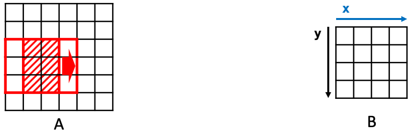
To analyze the data reuse, let’s take a closer look to the generated IR. To begin with, we can see that in two consecutive iterations of x (i.e., the inner loop), there are 6 pixels that are overlapped, as illustrated in the figure below. Without any optimization, we are reading 9 values from the input for each iteration.

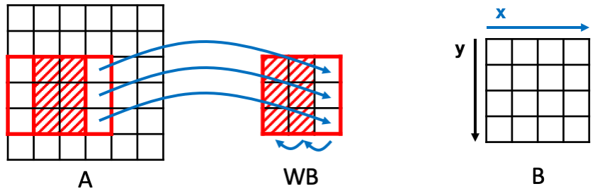
Introduce Data Reuse: Window Buffer

To reuse the overlapped pixels, we can introduce a reuse buffer. Since the filter moves like a window, we call the buffer a window buffer WB. The window buffers stores the reused pixels and also the new pixels that will be used in the current iteration. For each iteration, to update the values inside the window buffer, the last two columns, in this case, shift left. After that, the last column is replaced with the pixels read from the input. Now, we only read 3 values from the input for each iteration.

To introduce such reuse buffers in HeteroCL, we use the API reuse_at. The first argument is the tensor whose values will be reused. The second argument is the output stage that reuses the values of the tensor. The reason why we need to specify this is because we may have multiple stages reusing the values from the same input tensor. The third argument is the desired axis to be reused. It must be the output axis. Finally, we can specify the name of the reuse buffer. The API returns a new tensor.

s_x = hcl.create_schedule([A, F], kernel)
WB = s_x.reuse_at(A, s_x[kernel.B], kernel.B.axis[1], "WB")
print(hcl.lower(s_x))

Out:

// attr [_top] storage_scope = "global"
allocate _top[int32 * 1]
produce _top {
  // attr [0] extern_scope = 0
  produce B {
    // attr [WB] storage_scope = "global"
    allocate WB[int32 * 3 * 3]
    // attr [0] extern_scope = 0
    for (y, 0, 4) {
      for (x.reuse, 0, 6) {
        produce WB {
          for (A.1, 0, 3) {
            for (A.0, 0, 2) {
              WB[(A.0 + (A.1*3))] = WB[((A.0 + (A.1*3)) + 1)]
            }
            WB[((A.1*3) + 2)] = A[(x.reuse + ((y + A.1)*6))]
          }
        }
        if ((2 <= x.reuse)) {
          // attr [sum] storage_scope = "global"
          allocate sum[int32 * 1]
          produce sum {
            // attr [0] extern_scope = 0
            sum[0] = 0
          }
          for (ra2, 0, 3) {
            for (ra3, 0, 3) {
              sum[0] = int32((int65((int64(WB[(ra3 + (ra2*3))])*int64(F[(ra3 + (ra2*3))]))) + int65(sum[0])))
            }
          }
          B[((x.reuse + (y*4)) + -2)] = sum[0]
        }
      }
    }
  }
}

In the printed IR, you should be able to see a buffer WB with size (3, 3) being allocated. Moreover, in the produce WB scope, you should see the update algorithm described above. Now let’s test the function again.

hcl_Bx = hcl.asarray(np.zeros((4, 4)))
f = hcl.build(s_x)
f(hcl_A, hcl_F, hcl_Bx)
print('Output without WB:')
print(hcl_B)
print('Output with WB:')
print(hcl_Bx)

Out:

Output without WB:
[[361 230 167 161]
 [348 303 173 189]
 [302 269 234 221]
 [321 343 247 156]]
Output with WB:
[[361 230 167 161]
 [348 303 173 189]
 [302 269 234 221]
 [321 343 247 156]]

You should see the same results with and without the window buffer.

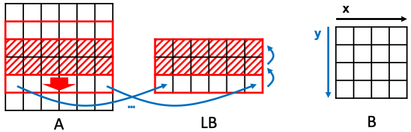
Reuse at a Different Dimension: Linebuffer

Similarly, we can create a reuse buffer for two consecutive iterations of y. In this case, in each iteration of y, we read an entire row from input A. Meanwhile, we update the reuse buffer by shifting up. Since it reads an entire line at a time, we call it a linebuffer LB. The operation is illustrated in the figure below.

Similar to the window buffer, we can introduce the linebuffer in HeteroCL by using a single reuse_at API. We show the code below.

s_y = hcl.create_schedule([A, F], kernel)
LB = s_y.reuse_at(A, s_y[kernel.B], kernel.B.axis[0], "LB")
print(hcl.lower(s_y))

hcl_By = hcl.asarray(np.zeros((4, 4)))
f = hcl.build(s_y)
f(hcl_A, hcl_F, hcl_By)
print('Output without LB:')
print(hcl_B)
print('Output with LB:')
print(hcl_By)

Out:

// attr [_top] storage_scope = "global"
allocate _top[int32 * 1]
produce _top {
  // attr [0] extern_scope = 0
  produce B {
    // attr [LB] storage_scope = "global"
    allocate LB[int32 * 3 * 6]
    // attr [0] extern_scope = 0
    for (y.reuse, 0, 6) {
      produce LB {
        for (A.0, 0, 6) {
          for (A.1, 0, 2) {
            LB[(A.0 + (A.1*6))] = LB[((A.0 + (A.1*6)) + 6)]
          }
          LB[(A.0 + 12)] = A[(A.0 + (y.reuse*6))]
        }
      }
      for (x, 0, 4) {
        if ((2 <= y.reuse)) {
          // attr [sum] storage_scope = "global"
          allocate sum[int32 * 1]
          produce sum {
            // attr [0] extern_scope = 0
            sum[0] = 0
          }
          for (ra4, 0, 3) {
            for (ra5, 0, 3) {
              sum[0] = int32((int65((int64(LB[((x + ra5) + (ra4*6))])*int64(F[(ra5 + (ra4*3))]))) + int65(sum[0])))
            }
          }
          B[((x + (y.reuse*4)) + -8)] = sum[0]
        }
      }
    }
  }
}

Output without LB:
[[361 230 167 161]
 [348 303 173 189]
 [302 269 234 221]
 [321 343 247 156]]
Output with LB:
[[361 230 167 161]
 [348 303 173 189]
 [302 269 234 221]
 [321 343 247 156]]

Note that the difference between WB and LB is the we reuse at different axes. We can also see from the printed IR that the allocated size is larger, which is the same as illustrated in the figure above. In this case, we read 6 pixels from the input for each iteration of y, which means we read 1 pixel for each iteration of x effectively. Namely, this is not true in terms of hardware execution. Can we do even better?

Combine Window Buffer and Linebuffer

We do not need to restrict ourselves to reuse at a single dimension. Since we have data reuse in both dimension, we can reuse both. In this case, we generate both a linebuffer and a window buffer. Let’s take a look at the figure first.

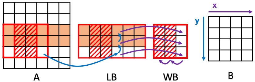
What happens here is that, we first update the linebuffer (blue arrows), then we update the window buffer (purple arrows). More precisely, for each iteration of x, we read 1 pixel from input ``A``. We simultaneously shift up the linebffer. After we update the linebuffer, we go on update the window buffer by reading pixels updated in the linebuffer. Then we shift the window buffer. To describe such behavior in HeteroCL is very easy. We only need to apply reuse_at twice. We just need to specify the corresponding reuse tensors and the reuse axes. In this case, the linebuffer reuses the pixels from the input A while the window buffer reuses from the linebuffer. Following we show the code and its IR.

s_xy = hcl.create_schedule([A, F], kernel)
LB = s_xy.reuse_at(A, s_xy[kernel.B], kernel.B.axis[0], "LB")
WB = s_xy.reuse_at(LB, s_xy[kernel.B], kernel.B.axis[1], "WB")
print(hcl.lower(s_xy))

hcl_Bxy = hcl.asarray(np.zeros((4, 4)))
f = hcl.build(s_xy)
f(hcl_A, hcl_F, hcl_Bxy)
print('Output without reuse buffers:')
print(hcl_B)
print('Output with reuse buffers:')
print(hcl_Bxy)

Out:

// attr [_top] storage_scope = "global"
allocate _top[int32 * 1]
produce _top {
  // attr [0] extern_scope = 0
  produce B {
    // attr [LB] storage_scope = "global"
    allocate LB[int32 * 3 * 6]
    // attr [WB] storage_scope = "global"
    allocate WB[int32 * 3 * 3]
    // attr [0] extern_scope = 0
    for (y.reuse, 0, 6) {
      for (x.reuse, 0, 6) {
        produce LB {
          for (A.1, 0, 2) {
            LB[(x.reuse + (A.1*6))] = LB[((x.reuse + (A.1*6)) + 6)]
          }
          LB[(x.reuse + 12)] = A[(x.reuse + (y.reuse*6))]
        }
        if ((2 <= y.reuse)) {
          produce WB {
            for (LB.1, 0, 3) {
              for (LB.0, 0, 2) {
                WB[(LB.0 + (LB.1*3))] = WB[((LB.0 + (LB.1*3)) + 1)]
              }
              WB[((LB.1*3) + 2)] = LB[(x.reuse + (LB.1*6))]
            }
          }
          if ((2 <= x.reuse)) {
            // attr [sum] storage_scope = "global"
            allocate sum[int32 * 1]
            produce sum {
              // attr [0] extern_scope = 0
              sum[0] = 0
            }
            for (ra6, 0, 3) {
              for (ra7, 0, 3) {
                sum[0] = int32((int65((int64(WB[(ra7 + (ra6*3))])*int64(F[(ra7 + (ra6*3))]))) + int65(sum[0])))
              }
            }
            B[((x.reuse + (y.reuse*4)) + -10)] = sum[0]
          }
        }
      }
    }
  }
}

Output without reuse buffers:
[[361 230 167 161]
 [348 303 173 189]
 [302 269 234 221]
 [321 343 247 156]]
Output with reuse buffers:
[[361 230 167 161]
 [348 303 173 189]
 [302 269 234 221]
 [321 343 247 156]]

We can see from the IR that the allocation sizes are indeed as expected.

Further Optimization

To further optimize the design, we need to think more carefully. For each iteration of x, there are three pixels in LB that are being read/write simultaneously. Thus, to maximize the memory bandwidth, we need to partition LB in the row direction. For WB, all pixels are updated at the same time. Therefore, we need to partition the whole WB completely. Finally, we can pipeline the whole design. Don’t forget that we also need to partition the filter F.

s_final = hcl.create_schedule([A, F], kernel)
LB = s_final.reuse_at(A, s_final[kernel.B], kernel.B.axis[0], "LB")
WB = s_final.reuse_at(LB, s_final[kernel.B], kernel.B.axis[1], "WB")
s_final.partition(LB, dim=1)
s_final.partition(WB)
s_final.partition(F)
s_final[kernel.B].pipeline(kernel.B.axis[1])
print(hcl.lower(s_final))

Out:

array partition variable=F complete factor=0 dim=0
// attr [_top] storage_scope = "global"
allocate _top[int32 * 1]
produce _top {
  // attr [0] extern_scope = 0
  produce B {
    // attr [LB] storage_scope = "global"
    allocate LB[int32 * 3 * 6]
    array partition variable=LB complete factor=0 dim=1
    // attr [WB] storage_scope = "global"
    allocate WB[int32 * 3 * 3]
    array partition variable=WB complete factor=0 dim=0
    // attr [0] extern_scope = 0
    for (y.reuse, 0, 6) {
      pipelined "initiation_interval"=1 (x.reuse, 0, 6) {
        produce LB {
          for (A.1, 0, 2) {
            LB[(x.reuse + (A.1*6))] = LB[((x.reuse + (A.1*6)) + 6)]
          }
          LB[(x.reuse + 12)] = A[(x.reuse + (y.reuse*6))]
        }
        if ((2 <= y.reuse)) {
          produce WB {
            for (LB.1, 0, 3) {
              for (LB.0, 0, 2) {
                WB[(LB.0 + (LB.1*3))] = WB[((LB.0 + (LB.1*3)) + 1)]
              }
              WB[((LB.1*3) + 2)] = LB[(x.reuse + (LB.1*6))]
            }
          }
          if ((2 <= x.reuse)) {
            // attr [sum] storage_scope = "global"
            allocate sum[int32 * 1]
            produce sum {
              // attr [0] extern_scope = 0
              sum[0] = 0
            }
            for (ra8, 0, 3) {
              for (ra9, 0, 3) {
                sum[0] = int32((int65((int64(WB[(ra9 + (ra8*3))])*int64(F[(ra9 + (ra8*3))]))) + int65(sum[0])))
              }
            }
            B[((x.reuse + (y.reuse*4)) + -10)] = sum[0]
          }
        }
      }
    }
  }
}

Finally, we can generate the HLS code and see if the II is indeed 1.

f = hcl.build(s_final, target="vhls")

Following is a sample report from Vivado_HLS.

+ Latency (clock cycles):
    * Summary:
    +-----+-----+-----+-----+---------+
    |  Latency  |  Interval | Pipeline|
    | min | max | min | max |   Type  |
    +-----+-----+-----+-----+---------+
    |   42|   42|   43|   43|   none  |
    +-----+-----+-----+-----+---------+

    + Detail:
        * Instance:
        N/A

        * Loop:
        +----------+-----+-----+----------+-----------+-----------+------+----------+
        |          |  Latency  | Iteration|  Initiation Interval  | Trip |          |
        | Loop Name| min | max |  Latency |  achieved |   target  | Count| Pipelined|
        +----------+-----+-----+----------+-----------+-----------+------+----------+
        |- Loop 1  |   40|   40|         6|          1|          1|    36|    yes   |
        +----------+-----+-----+----------+-----------+-----------+------+----------+

Limitations

Following we list the limitations of using reuse buffers in HeteroCL.

1. We do not accept non-linear index patterns, e.g., y*y+c, y*(y+c)

2. The stride is not one, e.g., 2*y+c

3. There is no overlapped pixel between two consecutive iterations of the specified axis, e.g., [x+r, y] and reuse y

More Examples: 2D Image Blur

HeteroCL is also able to infer reuse buffers for explicit reduction operations. Namely, instead of using hcl.sum, we can expand the compute patterns. Following is an example of 2D blur.

hcl.init()
A = hcl.placeholder((10, 10), "A")

def kernel_blur(A):
    return hcl.compute((8, 8), lambda y, x: A[y, x] + A[y+1, x+1] + A[y+2, x+2], "B")

s_blur = hcl.create_schedule(A, kernel_blur)
B = kernel_blur.B
RB_y = s_blur.reuse_at(A, s_blur[B], B.axis[0], "RB_y")
RB_x = s_blur.reuse_at(RB_y, s_blur[B], B.axis[1], "RB_x")
print(hcl.lower(s_blur))

Out:

// attr [_top] storage_scope = "global"
allocate _top[int32 * 1]
produce _top {
  // attr [0] extern_scope = 0
  produce B {
    // attr [RB_y] storage_scope = "global"
    allocate RB_y[int32 * 3 * 10]
    // attr [RB_x] storage_scope = "global"
    allocate RB_x[int32 * 3 * 3]
    // attr [0] extern_scope = 0
    for (y.reuse, 0, 10) {
      for (x.reuse, 0, 10) {
        produce RB_y {
          for (A.1, 0, 2) {
            RB_y[(x.reuse + (A.1*10))] = RB_y[((x.reuse + (A.1*10)) + 10)]
          }
          RB_y[(x.reuse + 20)] = A[(x.reuse + (y.reuse*10))]
        }
        if ((2 <= y.reuse)) {
          produce RB_x {
            for (RB_y.1, 0, 3) {
              for (RB_y.0, 0, 2) {
                RB_x[(RB_y.0 + (RB_y.1*3))] = RB_x[((RB_y.0 + (RB_y.1*3)) + 1)]
              }
              RB_x[((RB_y.1*3) + 2)] = RB_y[(x.reuse + (RB_y.1*10))]
            }
          }
          if ((2 <= x.reuse)) {
            B[((x.reuse + (y.reuse*8)) + -18)] = int32((int34((int33(RB_x[0]) + int33(RB_x[4]))) + int34(RB_x[8])))
          }
        }
      }
    }
  }
}